
Aug 08, 2019
Tobi Knaup
D2iQ

5 min read
Jupyter Notebooks—one of the industry’s favorite open-source web applications for creating and sharing documents housing live code, equations, visualizations, and more—are great for iterative data science work.
However, working with large datasets can be challenging since data doesn’t typically fit on the local disk or into local memory. Instead, data is stored in a cluster and a distributed computing framework such as Apache Spark is required to process it within a reasonable amount of time.
Now, this is where BeakerX comes in.
BeakerX is a collection of Jupyter kernels and notebook extensions that allows you to work efficiently with large Spark datasets directly from a notebook. In addition, you can still use the data science libraries you're familiar with for local development.
In this tutorial, you’ll learn how to use BeakerX to build an interactive notebook that reads a dataset from HDFS and classifies the data using a linear model built with Spark in Scala. We’ll also produce a report using popular Python libraries.
Before we dive in, it’s important to note that this tutorial assumes you're using Jupyter Notebooks on DC/OS, which offers notebooks preconfigured with many popular data science tools such as Spark, BeakerX, pandas, and scikit-learn.
How to Build an Interactive Spark Notebook
Step 1: Prepare your Cluster
To run this tutorial you need the HDFS and Jupyter packages installed on your DC/OS cluster. Directions for installing HDFS and configuring Jupyter can be found in this tutorial video.
Once you have these packages installed, navigate to your Jupyter instance and open a terminal tab. Then, run the following command from the Jupyter terminal to clone the repository that contains the notebook for this tutorial:
git clone https://github.com/dcos-labs/data-science.git
Using the Jupyter file browser, navigate to the folder called data-science and then to beakerx. Once there, open the notebook called BeakerX.ipynb.
Step 2: Using an Interactive UI to Select Input Parameters
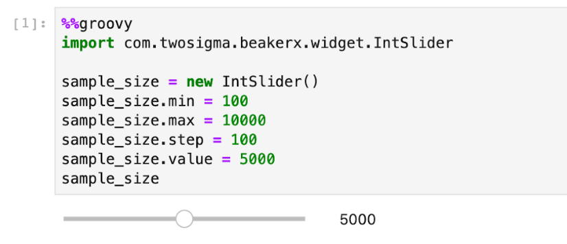
The code below renders a slider that we can use to change the value of sample_size, which will be used further down. UI components are a great way to produce interactive notebooks that make data exploration more engaging and BeakerX offers a number of forms, widgets, and interactive components.
Notice the %%groovy magic on the first line. This tells BeakerX to interpret the cell content using the Groovy programming language. BeakerX supports multiple languages per notebook this way, allowing users to take advantage of the best tools for the job—even if they're in different programming languages.
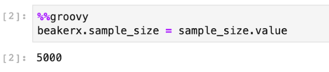
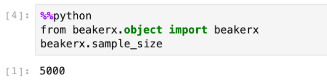
The next cell demonstrates how to use the BeakerX Autotranslation feature. This feature allows you to synchronize data between cells that are written in different programming languages. Assigning the value to the BeakerX object allows us to read it back in other languages later.
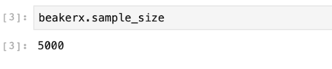
Now, we can easily read the value of sample_size from the default language of this notebook, which is Scala.
It’s also available in other languages such as Python. For more examples in additional languages, see the docs for Autotranslation.
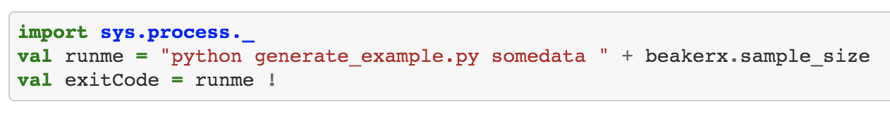
Now, we’ll use the sample size given above to generate a set of records and load them into HDFS. This cell outputs the exit code of the script, which should be “0” on success.
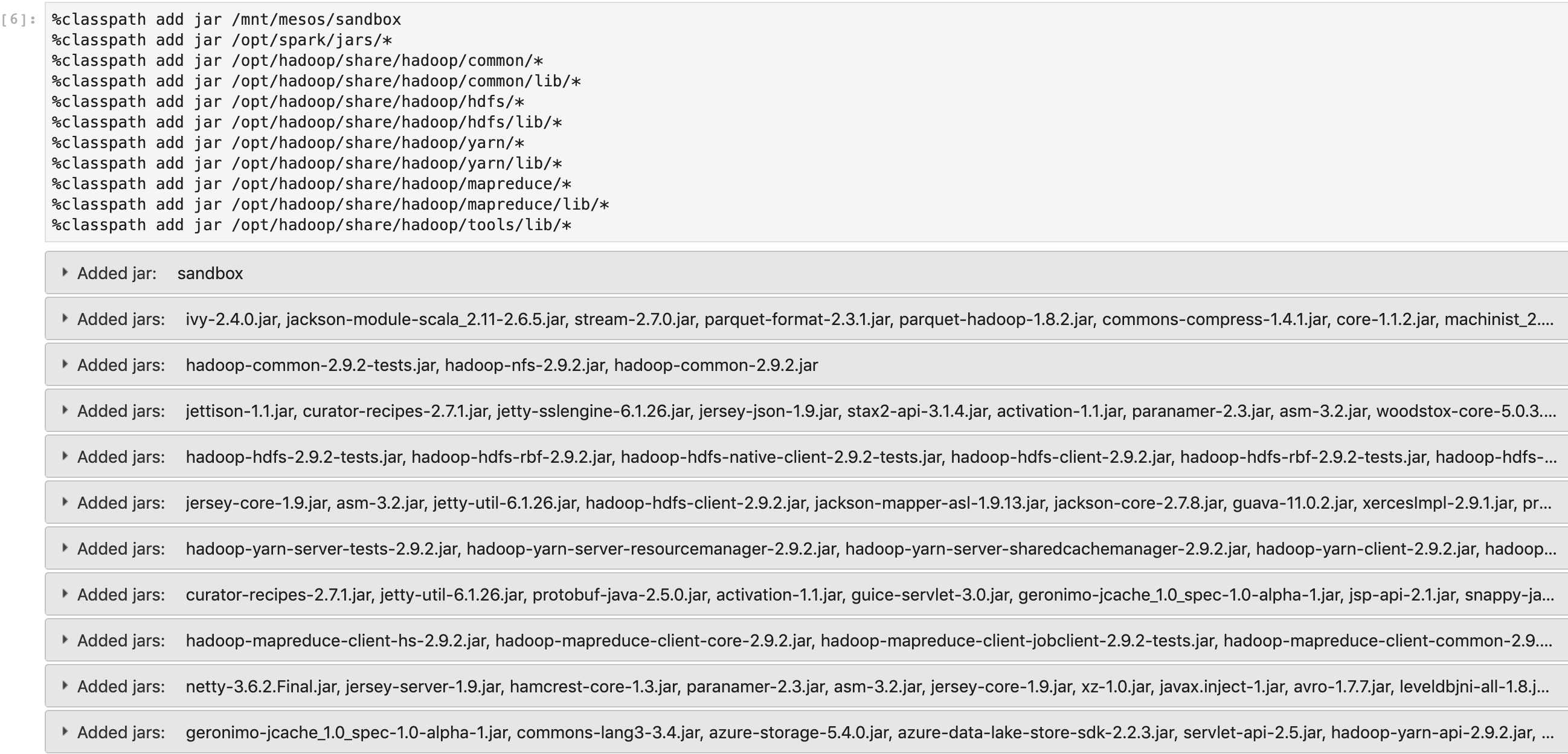
Step 3: Adding Spark and Hadoop Libraries
The Jupyter package includes the Spark and Hadoop JARs that we need to run our Spark job. So, you don't need to download them from the internet. Now, let’s add them to the classpath.
Step 4: Using the BeakerX GUI to Run Spark Jobs
To run distributed Spark jobs on DC/OS using the BeakerX Spark UI, we need to change some of the default settings. Run the cell below and once the UI loads make the following changes:
- Remove the setting for spark.mesos.principal by clicking the “X” next to it
- Change the value for spark.mesos.executor.docker.image to mesosphere/mesosphere-data-toolkit:1.0.0-1.0.0
- Click “Save”
Once this is done, hit “Start” to launch a Spark cluster directly from this notebook. Depending on the specs of your cluster, this will take anywhere from a few seconds to a few minutes. Once it's ready, you'll see a star-shaped Spark logo on a green label button, along with additional buttons.
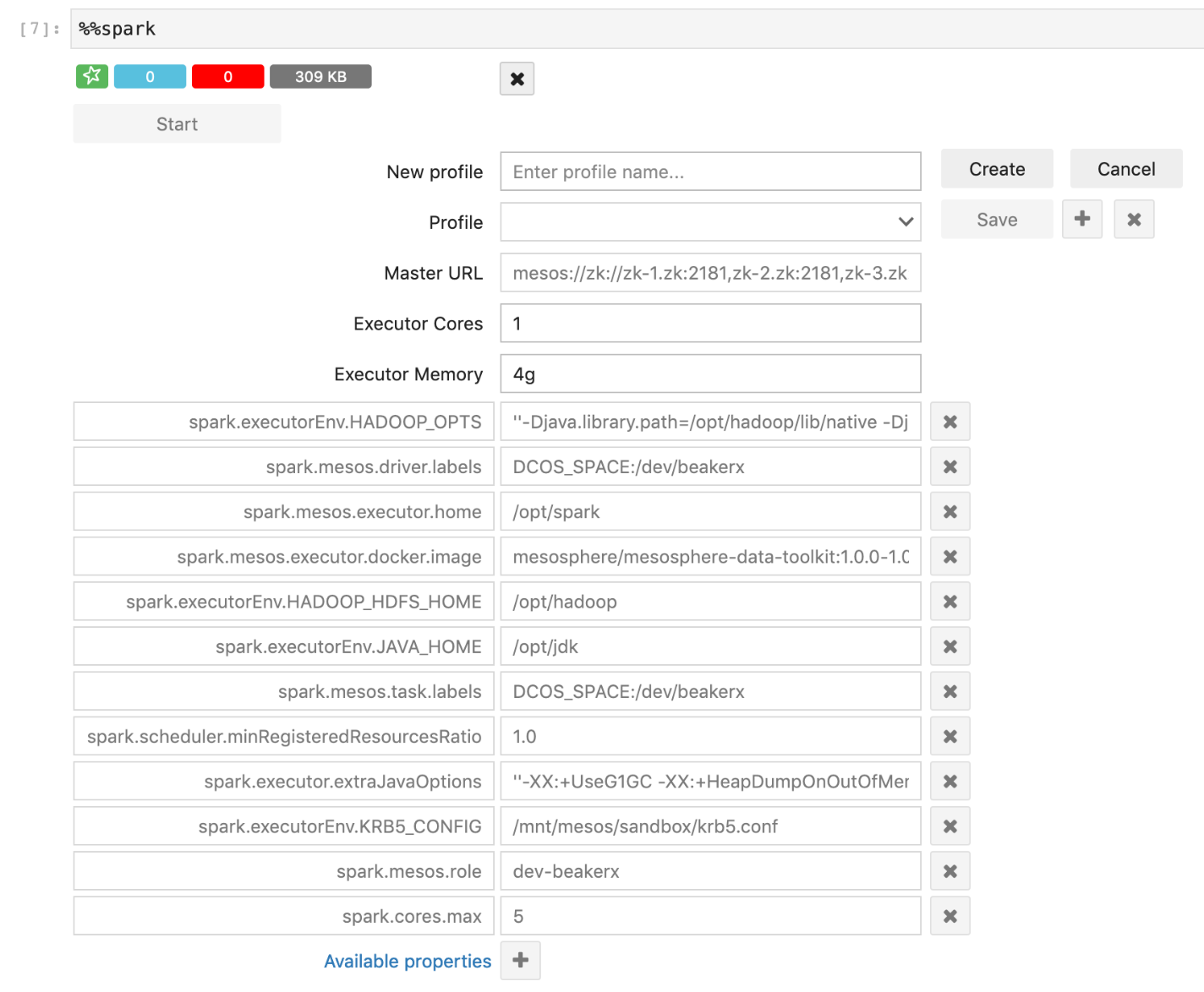
The GUI provides useful metrics for working with Spark and allows you to track the progress of your jobs. It also allows you to easily create, save, and select multiple configurations. You can jump directly to the Spark UI by clicking the green Spark logo.
Step 5: Run a Spark Job
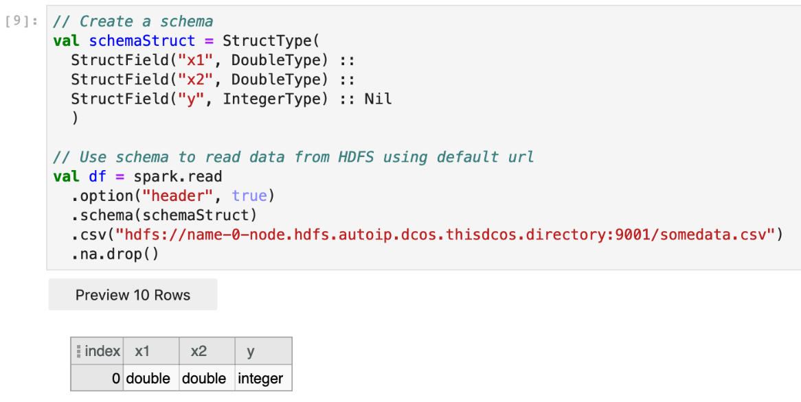
Now, let's write the Spark job that builds a linear model for our dataset. First, we need to import its dependencies.
Next, we need to load the data from HDFS that was generated previously.
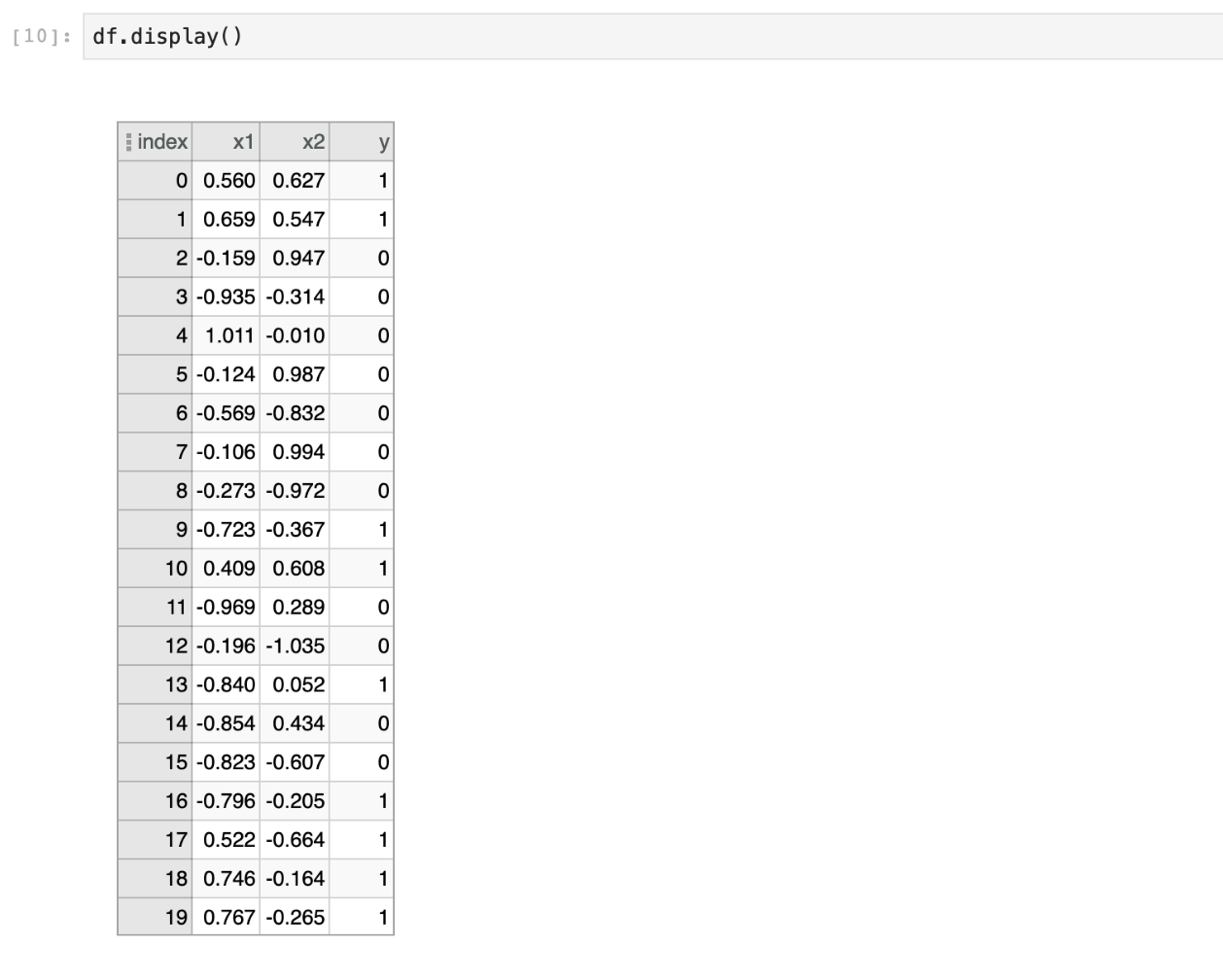
Once this is complete, display the results with a table view using df.display(). This will trigger the Spark job and a progress bar will appear. You can click on the ellipses in the column headers for filtering, sorting, and other options.
Next, we’ll run a logistic regression and get results. The output of this cell is the model accuracy.
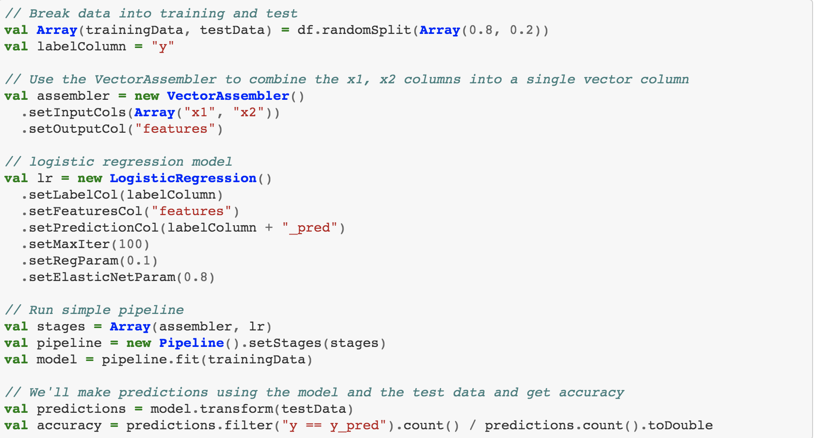
The accuracy is only about 0.5, which is equivalent to flipping a coin, so our model isn't very good.
Step 6: Debug Model Performance
Let's find out why our model performed so poorly by plotting the data.
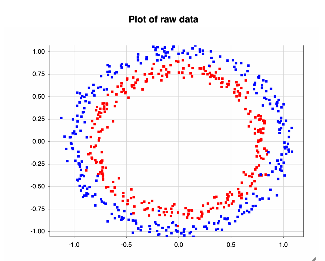
The data is plotted in a circle. So, it’s easy to see why a linear partition won't split the positive and negative cases. Using the Pythagorean Theorem, we can map the data into something we can linearly split.
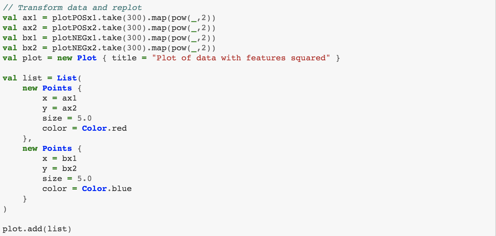
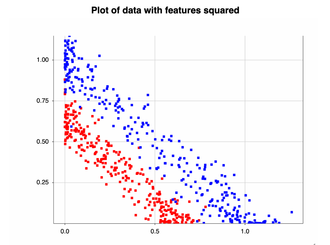
This should be easy for a logistic regression to classify. Let's redo the model with the transformed data and output the accuracy.
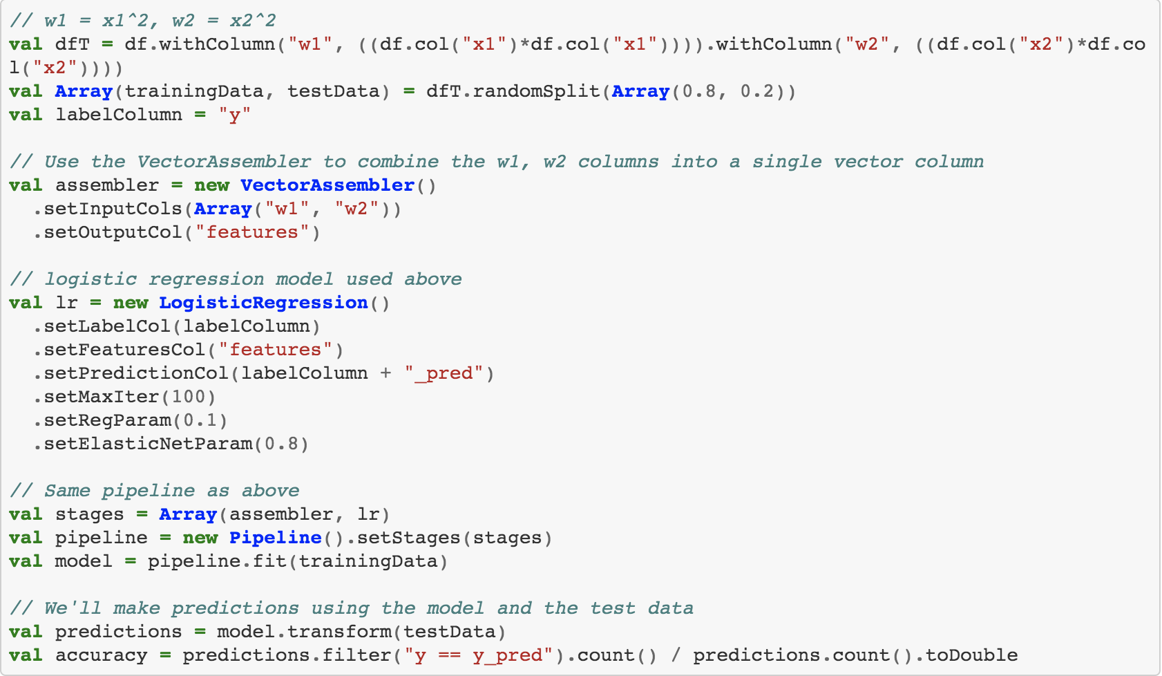

As expected, the model works much better, with accuracy being close to 1.0.
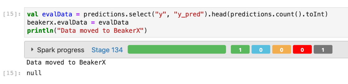
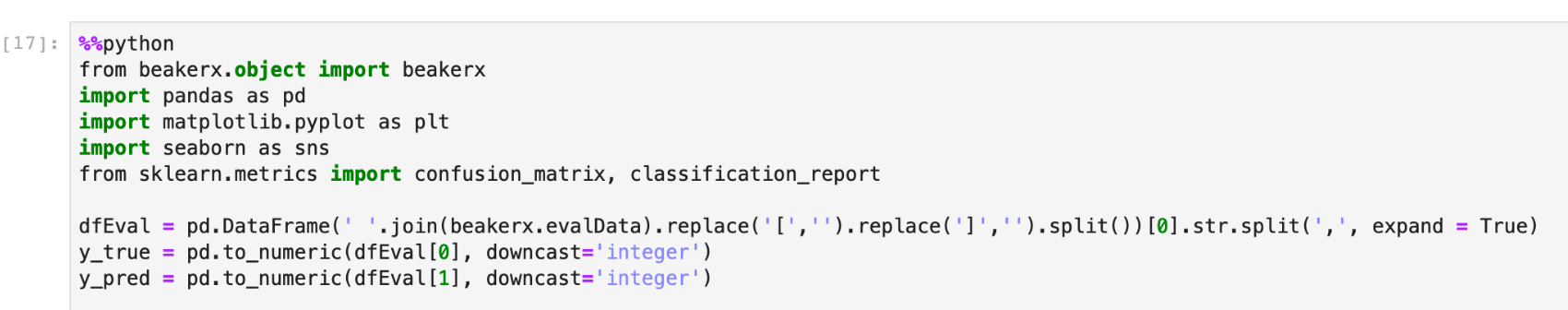
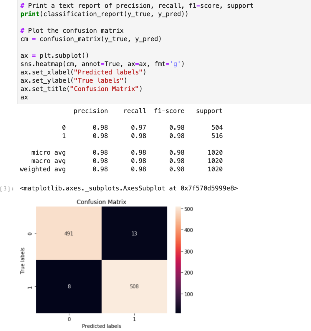
But accuracy is only one useful metric. A confusion matrix will give us more details on how our model performed. You can easily create one using scikit-learn, which is a Python library included in the Jupyter package. We can use the BeakerX Autotranslation feature again to pass the data to Python.
Now the data is accessible from Python and we can build and plot our confusion matrix using scikit-learn.
What Did We Learn Today?
In this tutorial, we learned how to create an interactive UI within a notebook to read input parameters from a user. We then launched Spark jobs and tracked their progress using the BeakerX Spark UI without leaving the notebook environment. Lastly, we used multiple programming languages in a single notebook and easily synchronized data between them using BeakerX Autotranslation.
Looking for more helpful tutorials or resources? Check out our other tutorials on this blog and our robust resource center featuring videos, eBooks, whitepapers, infographics, and more.