
Mar 28, 2018
Chris Gutierrez
D2iQ

9 min read
TensorFlow is a popular open source library for machine learning. It was the #1 most forked GitHub project of 2015. Its popularity stems from its ability to simplify the development and training of deep neural networks using a computational model based on data flow graphs. A longer description of TensorFlow and a rundown of the features that simplify its installation and management on DC/OS can be found here.
Setting up and running TensorFlow for development on a laptop isn't difficult. Setting up TensorFlow for development that matches production, however, can be more of a challenge. Typically, a team of data scientists works on the same production cluster, but each data scientist requires a particular configuration and Python library. Setting up unique requirements on the same cluster is time-intensive for both operators and data scientists. DC/OS can turn it into a point-and-click installation process while remaining flexible on use cases. With DC/OS the laptop or staging environment can be set up similar enough to production that migrating code and data back and forth is trivial.
This blog post assumes you have a DC/OS cluster up and running. You can follow this tutorial about DC/OS advanced installation or consult DC/OS installation documentation for directions to install DC/OS on a laptop, AWS, Azure, or GCE.
There are many Integrated Development Environments (IDE) that can be used to write TensorFlow or Python code. Among the most common are Jupyter Notebooks. Jupyter Notebooks allow users to create and share documents that contain live code, equations, visualizations and narrative text. There are entire systems built around Jupyter Notebooks to help with code collaboration. Jupyter is the IDE of choice for many data scientists for many reasons, and BeakerX is basically Jupyter Notebooks on steroids.
Data scientists have a demanding job to do: connecting and combining billions of records from multiple data sources and performing complex analyses. BeakerX streamlines and accelerates this process by connecting to multiple data sources to manipulate, explore, and model that data, eventually deploying an operating model into production.
What is BeakerX?
BeakerX is a collection of kernels and extensions to the Jupyter interactive computing environment. It provides JVM support, interactive plots, tables, forms, publishing, and more. BeakerX was created and open-sourced by Two Sigma, an investment company that applies the scientific method to investment management, combining massive amounts of data, world-class computing power, and financial expertise to develop sophisticated trading models. Two Sigma is deeply committed to developing, improving, and sharing open source software.
Mesosphere has been working with Two Sigma for many years, primarily on building solutions for managing Two Sigma's clustered compute environments. David Palaitis, SVP at Two Sigma describes how Apache Mesos facilitates data science in their environment, saying that "it's nice to be working further up the stack now - extending Mesosphere DC/OS with an Integrated Development Environment (IDE) for data scientists. The IDE, built on Jupyter and BeakerX, abstracts the complexity of managing distributed compute. Beyond that, it makes it easier to manage the rich data analysis and machine learning software stacks required to practice data science at scale today. We're looking forward to releasing more functionality for dataset discovery, notebook sharing and Spark cluster management into the open source BeakerX product later this year."
BeakerX supports:
- Polyglot Analysis: Groovy, Scala, Clojure, Kotlin, Java, and SQL, including many magics
- Widgets: time-series plotting, tables, forms, and more (there are Python and JavaScript APIs in addition to the JVM languages)
- Collaboration: One-click publication with interactive plots and tables
- Jupyter Lab
Installing BeakerX on DC/OS
BeakerX is preinstalled in the DC/OS JupyterLab framework. The JupyterLab framework can be installed on DC/OS with a point-and-click interface. To help you get started, a simple installation walkthrough follows. More thorough documentation and BeakerX source code can be found here.
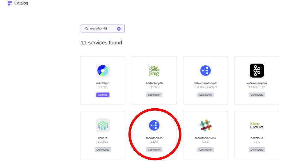
DC/OS Service Catalog
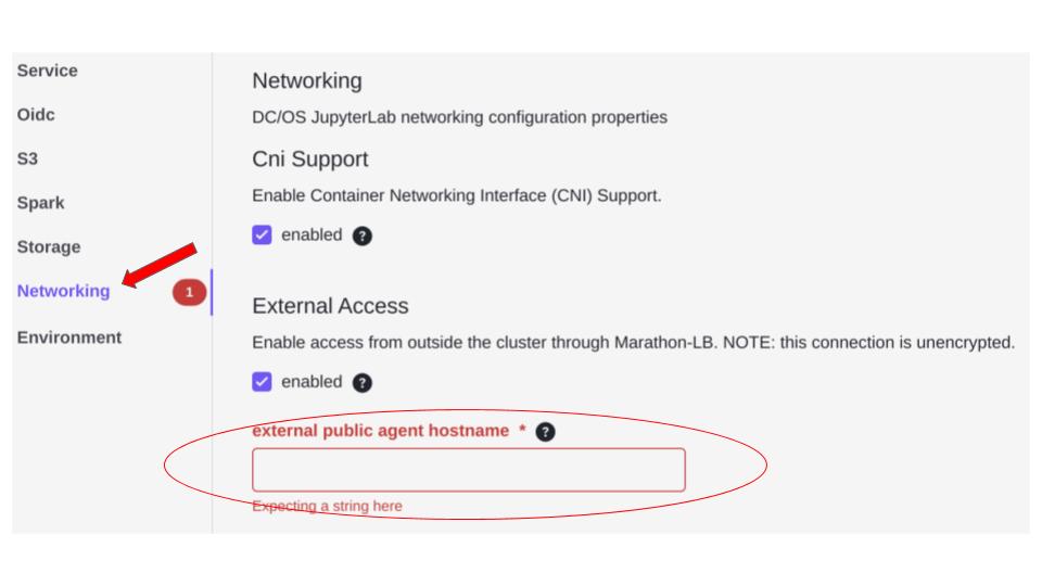
First, a load balancer accessible outside the cluster must be installed. Find marathon-lb in the DC/OS Service Catalog and click it to begin the installation. A menu will open that allows you to review and change container settings before starting the container. The default settings will get you started quickly, but they can be adjusted based on your needs.
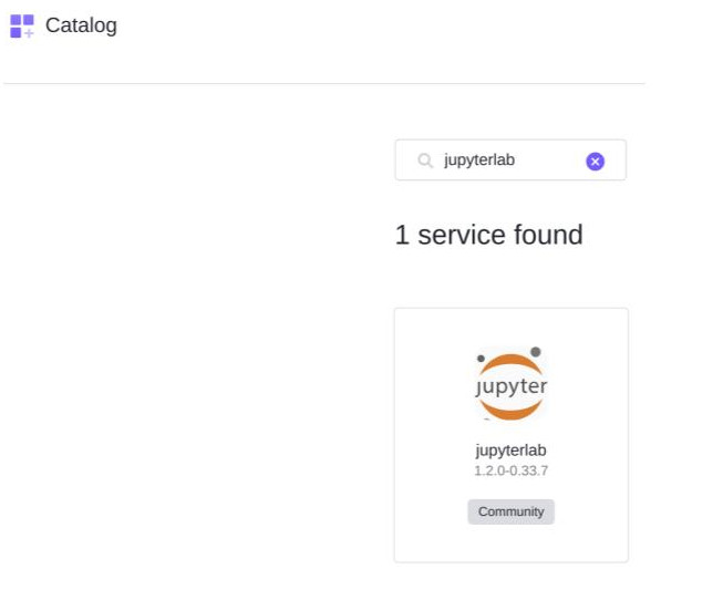
Next, find JupyterLab in the DC/OS Service Catalog, double-click it to begin the installation. In this case, edits are required to the configuration prior to installation.
Edit the Networking section. The external public agent hostname must point to the marathon-lb load balancer just setup. You should know the agent address from the DC/OS install. Paste the public agent address into the external public agent hostname for JupyterLab.
Running JupyterLab with BeakerX
Go to public <agent address>/jupyterlab-notebook.
Working with a Simple Neural Net in BeakerX
Before we begin, we'll need to load some data. Often the data is on your laptop. While generally not difficult, it's often tedious getting data from a laptop to a cluster. A common approach is to copy a file to an externally reachable node, and then sometimes it's required to copy the file to another node and then finally into the container. With the notebook, however, it's simple. Just hit "upload", find the file on the laptop and upload it. Another advantage of BeakerX is that it's easy to work with "real," i.e., large datasets. The code can be inside BeakerX, while the execution can complete on a scalable solution (e.g., Spark, Cassandra, etc.). For simplicity, we'll cheat and use a dataset that is publicly readable (The code below are snippets from this notebook code).
from keras.models import Sequentialfrom keras.layers import Denseimport tensorflow as tsimport pandas as pdimport numpy as npimport sklearn.model_selection as skfrom beakerx import *df = pd.read_excel('http://biostat.mc.vanderbilt.edu/wiki/pub/Main/DataSets/titanic3.xls', 'titanic3', index_col=None, na_values=['NA'], converters={'ticket':str})[['sex','age','name','cabin','ticket','survived']]table = TableDisplay(df)table.setStringFormatForTimes(TimeUnit.DAYS)table.setStringFormatForType(ColumnType.Double, TableDisplayStringFormat.getDecimalFormat(4,6))table.setStringFormatForColumn("m3", TableDisplayStringFormat.getDecimalFormat(0, 0))table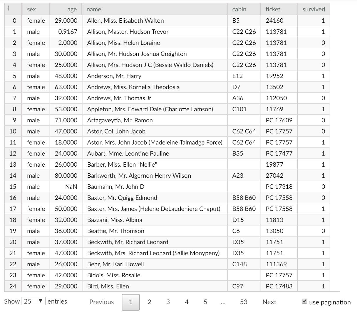
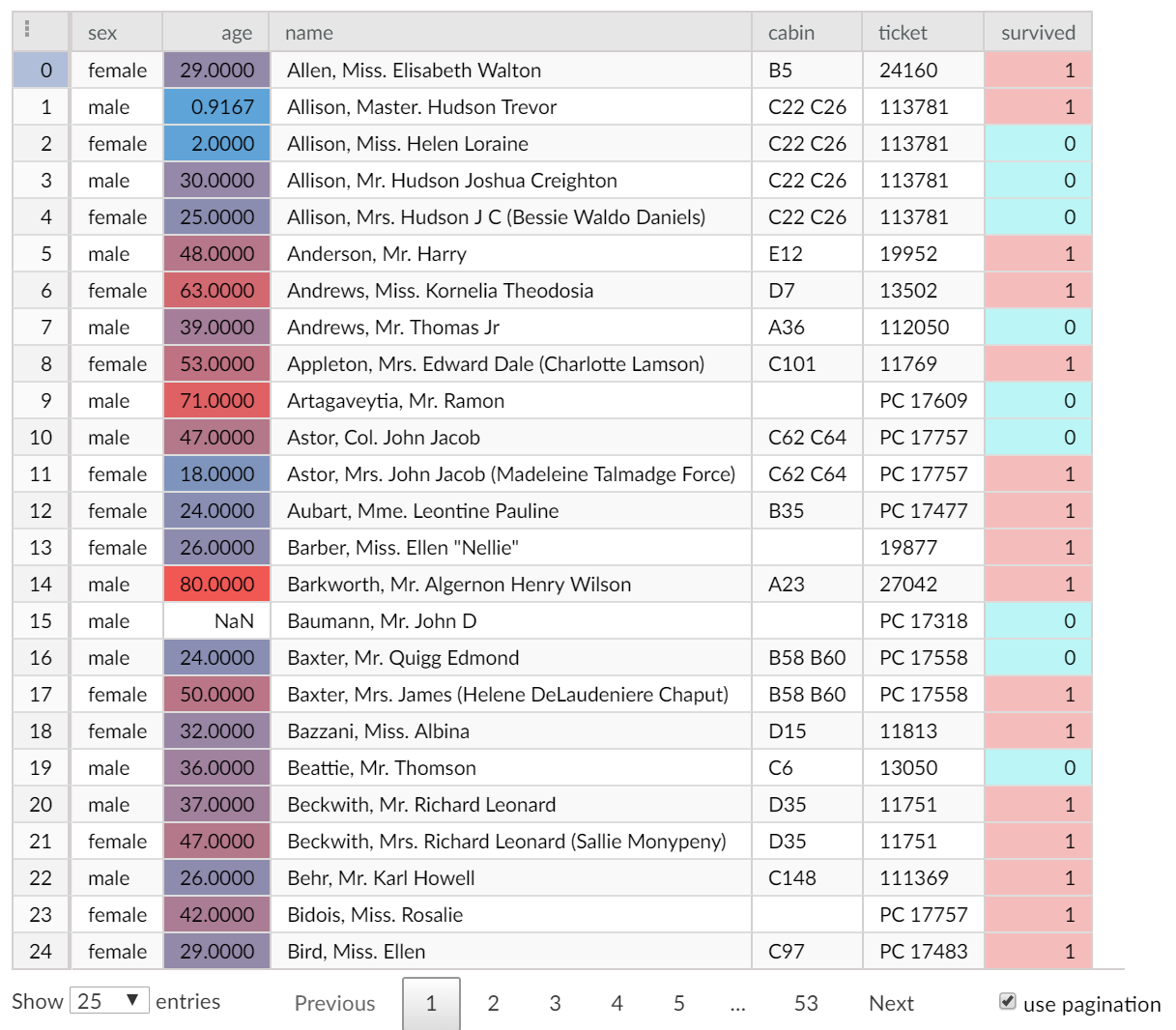
The first phase of any data science project is to identify and inspect the working datasets. For smaller datasets, this can be done using off the shelf offerings. However, as datasets get larger and wider, advanced table capabilities can really help to make analysis efficient. BeakerX includes a full set of table capabilities that have been informed by many years of developing solutions for Two Sigma's data scientists. The result is an interactive table with many options.
Using the BeakerX TableWidget, you can color by unique value, create heatmaps, and more.
After inspecting data in tabular form, a data scientist might start to visualize and explore the data to learn more. BeakerX includes an interactive plotting API that is designed from the ground up for dataset visualization. The example below shows an interactive plot comparing male vs. female survival rate over time.
x = df.loc[:,['survived', 'sex']]x['age'] = df.loc[:, 'age'].round(-1)m_mean = x.query('age>=0 & age<70 & sex=="male"').groupby(['age']).mean()m_std = x.query('age>=0 & age<70 & sex=="male"').groupby(['age']).std() m_low = m_mean - m_stdm_hi = m_mean + m_std f_mean = x.query('age>=0 & age<70 & sex=="female"').groupby(['age']).mean() f_std = x.query('age>=0 & age<70 & sex=="female"').groupby(['age']).std()f_low = f_mean - f_stdf_hi = f_mean + f_stdp = Plot()p.add(Line(y= f_mean.survived, displayName= "Female Survival Rate"))p.add(Area(y= f_low.values.tolist(), base= f_hi.values.tolist(), color= Color(0, 30, 0, 0), displayName= "1 Standard Deviation Female"))p.add(Line(y= m_mean.survived, displayName= "Male Survival Rate"))p.add(Area(y= m_low.values.tolist(), base= m_hi.values.tolist(), color= Color(255, 0, 0, 50), displayName= "1 Standard Deviation Male"))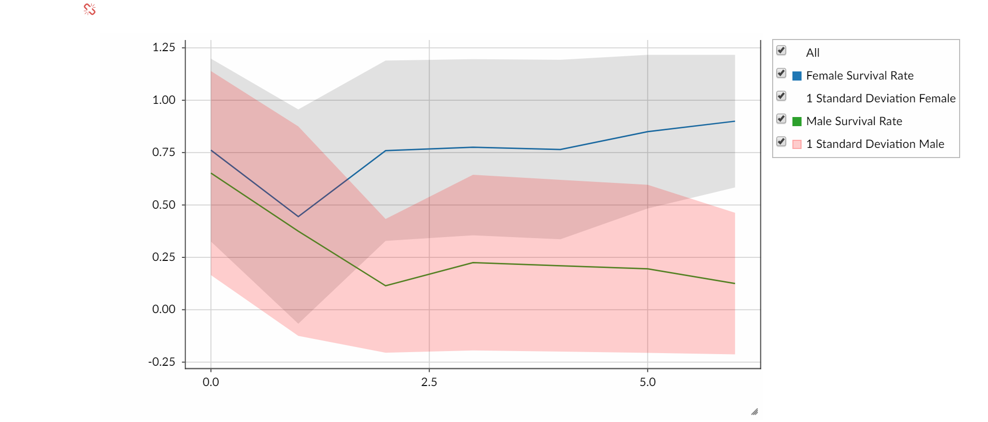
After visualizing and building an intuition for the data, a data scientist will typically form a hypothesis about the predictive power of the data, then build, train, and test a model to validate the hypothesis. We'll build a model to test the hypothesis that the "title" of a passenger on the Titanic can help predict whether they survived or not. The title is not available as a column in the dataset, but it can be extracted from the name of the passenger. The title is information-rich and might have as much predictive power than sex, age, or cabin combined. The example below uses the Tensorflow library to build a neural network to test this hypothesis. While a full explanation of what's happening here is beyond the scope of this document; there are plenty of TensorFlow online tutorials and you can read more about TensorFlow on DC/OS. We include this example to show the powerful combination of BeakerX and TensorFlow.
First, let's do some data pre-processing to extract the ‘title' feature.
# pandas and regex magic to extract the title of the passenger into a 'title' columndf['title'] = df['name'].str.extract('.*, (.*).', expand=False)x_all = pd.get_dummies(df['title'])y_all = np.array([ [y==1, y==0] for y in df.survived]).astype(int)Now, split the data into a training set and a test set.
X_train, X_test, y_train, y_test = sk.train_test_split(x_all, y_all, test_size=0.33, random_state=42)
Next, we use the high-level Keras API for TensorFlow to build and compile a simple neural network.
model = Sequential()model.add(Dense(units=32, input_dim = len(x_all.columns)))model.add(Dense(units=32, input_dim = len(x_all.columns)))model.add(Dense(units=2, activation='softmax'))model.compile(loss='categorical_crossentropy', optimizer='sgd', metrics=['accuracy'])
The model can be used to predict the survival status of passengers in the test data.
predictions = model.predict(X_test.as_matrix())
Finally, we can calculate a simple score for our model.
# assign the softmax probabilities to a boolean e.g. true or falsepredictions_bool = predictions[:,0] > 0.5# do the same for the responsey_test_bool = y_test[:,0] ==1accuracy = sum(predictions_bool == y_test_bool) / len(y_test_bool)
78%. Not great, but not bad for only using the 'title' feature data!
The basics have been covered so we'll leave further analysis to you. The interactive nature of BeakerX will significantly reduce the time to identify problems in this model and make improvements.
BeakerX on DC/OS: Data Science at Scale
The above model is only an example to introduce you to working with BeakerX and TensorFlow. DC/OS has packages for Apache HDFS, Apache Spark, and many NoSQL and traditional RDBMS databases. A real-world data science problem could potentially connect and combine billions of records from multiple data sources. A BeakerX notebook could connect to those data sources to manipulate, explore and eventually model that data. The final step would be to push a real model into production. Fortunately, anything done with TensorFlow can be accessed with TensorFlow Serving. We'll save that for its own blog post.
If you have a favorite data manipulation or modeling software that isn't already in the DC/OS Service Catalog, it's easy to add it yourself. Simply put it into a Docker container and add it to DC/OS. Most importantly, if you can access it with Python, then you can access it with BeakerX. DC/OS allows you to mix and match solutions while BeakerX gives you an easy interface to work with those solutions.